
Artificial intelligence is often described as learning a model from data. That is one important family of approaches, not a universal definition of intelligence. In weather, oceanography, energy systems, industrial processes and many other physical domains, equations, conservation laws, boundary conditions and decades of scientific knowledge already exist. The real challenge is frequently to combine that knowledge with observations that are sparse, noisy and incomplete.
01 A forecast can obey every equation and still start from the wrong world
A dynamical model describes how a system evolves from an initial state. Write it as dx/dt = F(x) with x(0) = x₀, where the state vector x(t) lives in ℝⁿ. If that initial state x₀ is wrong, the model can solve its equations perfectly and still produce the wrong trajectory. In nonlinear systems such as the atmosphere or the ocean, small errors in the starting state grow quickly — the defining property of deterministic chaos, and the reason a forecast is only ever as good as its initialisation.
Observations do not solve the problem by themselves. Satellites, buoys, radars and sensors measure only selected variables, at selected places and times, with uncertainty. The complete model state may contain millions of values; the observation vector is usually far smaller. Recovering the full, physically consistent state from those fragments is not interpolation — it is inference under a constraint, where the constraint is the model itself.
The equations encode structure and physical consistency, yet the starting state and parameters may be uncertain.
Measurements anchor the model in reality, but they do not describe every variable or every point in space and time.
Infer the hidden initial condition, parameters or trajectory that best explains the evidence while respecting the model.
This is the territory of inverse problems, and it is worth being formal about it, because the course is. Mathematical modelling describes a system through equations — typically ordinary or partial differential equations — that involve parameters, initial conditions and boundary conditions. Solving them in the natural direction is the direct (or forward) problem: given the inputs and parameters, compute the output. Writing a model as a map M : (x, p) ↦ y from inputs x and parameters p to output y, the inverse problem is to run that map backwards: given partial knowledge of y, recover x and/or p. Inverse problems arise precisely when a system is only partially known but can be observed, and one wants to recover characteristics that are not directly measurable.
The applications are everywhere the course points: medical imaging (X-ray and ultrasound tomography, elastography), image analysis (deblurring, denoising, inpainting, restoration), geosciences (seismic tomography, radio-astronomical imaging, and data assimilation for weather forecasting), signal processing (deconvolution), and mechanical engineering (crack detection and other non-destructive testing). And there is a bridge to machine learning that the course makes explicitly: model fitting and parameter identification are inverse problems. Multivariate linear regression — recover the coefficient matrix A in y = Ax from observed pairs, in the least-squares sense — is the simplest one. The same framing covers neural-network training, and parameter estimation in ODE and PDE models, including the calibration of digital twins.
Why inverse problems are hard: Hadamard, and the instability of running a model backwards
In 1902 Jacques Hadamard introduced the notion of a well-posed problem. A problem is well-posed if three properties hold: a solution exists, the solution is unique, and the solution depends continuously on the data. If any of the three fails, the problem is ill-posed.
Existence and uniqueness are intuitive prerequisites — without uniqueness, even perfect data may not pin down what you want to recover. The third condition, stability, is the subtle and consequential one. It says that a small change in the data — typically measurement error — should produce only a small change in the reconstructed solution. Forward problems are usually stable; inverse problems, because they often run against irreversibility or causality, frequently are not. Ill-posedness is the rule, not the exception.
The course makes this concrete with the cleanest possible example: differentiation. Differentiating is the inverse of integrating, and it is unstable. Take a smooth function f and perturb it by a tiny high-frequency wiggle, f_δ,n(x) = f(x) + δ·sin(nx). The perturbation to the function has amplitude δ, which you can make as small as you like. But the perturbation to its derivative has amplitude δ·n, which grows without bound as the frequency n increases. An arbitrarily small error in the data produces an arbitrarily large error in the answer. Parameter identification in a differential equation behaves the same way: in the one-dimensional heat equation −d/dx(a(x)·du/dx) = f, recovering the unknown conductivity a from temperature measurements is straightforward to write down and yet ill-posed wherever the temperature gradient vanishes — there, no solution exists at all.
The practical consequence is regularisation: you add prior information to restore stability, trading a little fidelity to the noisy data for a solution that does not explode. That is not a trick bolted on at the end; it is a modelling decision about what you believe before you look. Holding onto that idea — that the choice of prior is a deliberate, inspectable assumption — is most of what separates a defensible reconstruction from a confident-looking artefact.
02 Data assimilation: make the model listen without making it forget
Data assimilation is the mathematical field at the interface of model and observation. It does not ask the data to replace the model, or the model to ignore the data. It asks for the state that makes the two as compatible as possible — a controlled negotiation in which the model contributes dynamics (which evolutions are physically possible), the observations contribute correction (where the simulated trajectory departs from reality), and a set of statistical assumptions decides how strongly each source should be trusted.
The course teaches the field as it actually exists: not one algorithm, but a small family of method classes, each with a different bargain between optimality, assumptions and cost.
A small assimilation laboratory
This deliberately simple illustration blends a model trajectory with observations. The teal analysis moves as the assumed confidence in the observations changes. Real data assimilation uses richer covariance structures, dynamical constraints and optimisation.
- Variational methods treat assimilation as minimising a cost function. 3D-Var finds the best state estimate at a single time; 4D-Var finds the best state estimate across an entire assimilation window, and is formulated through optimal-control theory. (3D-Var was the operational method at Météo-France until 2000 — a useful reminder that "state of the art" has a date on it.)
- Sequential methods alternate a forecast step with a statistical correction step. Optimal interpolation is easy to implement but physically incoherent; the Kalman filter is the theory of optimal statistical estimation; ensemble and reduced-order variants (EnKF, the SEEK filter) exist precisely because the full filter does not scale — more on that below.
- Nudging methods add a feedback term to the model equations, continuously pulling the simulated state towards the observations. They are, in control-theory language, observers — and they are where Blum and Auroux made their own contribution, the subject of §05.
The honest framing throughout is the same one the course insists on: a reconstructed state is only as good as the evidence and the mechanism behind it. Built carelessly, assimilation launders assumptions into conclusions. Built well, it is a way of reasoning rigorously about a system you cannot fully observe.
03 Optimisation is the bridge — and this is where the curriculum converges
Variational data assimilation turns reconstruction into an optimisation problem, and this is the precise point at which the school's optimisation course stops being a prerequisite box to tick and becomes the engine of the method. The 4D-Var cost function, in the notation the course uses, is
The mathematical details determine how errors are weighted and how uncertainty propagates. The core idea is a constrained search for the trajectory most consistent with both the equations and the measurements.
Simulate the system from the current estimate of the initial state.
Determine how changing the unknowns changes the mismatch.
Update the estimate, run again and continue until an acceptable solution is reached.
The unknowns are the initial state x₀ and the model parameters u. The first term keeps the solution close to a prior estimate x_b (the background), weighted by the inverse of the background-error covariance B. The second term penalises the gap between the model trajectory and the observations at each time tᵢ, weighted by the inverse of the observation-error covariance Rᵢ, with the observation operator Hᵢ mapping the model state into observation space. Minimising J subject to the model dx/dt = F(x, u) is exactly an optimal-control problem: find the initial condition and parameters that produce the trajectory most consistent with both the equations and the measurements.
Everything the Continuous Optimisation course builds is needed here. The cost function is a real-valued objective over a high-dimensional space; the model is a constraint; the covariance-weighted norms are quadratic forms; convexity (or its absence) decides whether a minimum is global; and the minimiser is found not by a closed-form inverse but by an iterative gradient method. At a single time, 3D-Var even admits the explicit solution x* = [B⁻¹ + HᵀR⁻¹H]⁻¹(B⁻¹x_b + HᵀR⁻¹x_obs) — and the course is careful to point out why that formula is useless in practice: the matrices are far too large to invert, so one evaluates J and its gradient and hands them to an optimisation algorithm instead.
That raises the question the whole method turns on: how do you get the gradient of J with respect to a control vector that may have tens of millions of components? Finite differences would require one model run per component — utterly impossible. The answer is the adjoint method: run the forward model once, then integrate an adjoint model backward through the window, picking up a forcing term at each observation time, and read the full gradient off the adjoint solution. The cost is one forward solve plus one backward solve, independent of the dimension of the control vector. That single fact is what makes large-scale variational assimilation feasible at all.
The course does not hide how demanding this is, and two of its warnings are worth surfacing, because they are exactly the kind of detail that separates a working system from a plausible one:
- The adjoint of the discretised model is not the discretisation of the continuous adjoint. Deriving the adjoint equations on paper and then discretising them gives the wrong gradient; the correct route is to differentiate the discrete model directly (in practice, via automatic differentiation — tangent-linear for the forward derivative, adjoint for the reverse). "Differentiate, then discretise" and "discretise, then differentiate" do not commute, and getting this backwards is a classic, silent source of error.
- For a nonlinear model,
Jis generally not convex. It can have multiple local minima, so the result depends on where the optimisation starts, and a regularisation term —α‖x₀ − x₀_background‖² + β‖u − u_background‖²— is added to tame the problem. Large coefficients penalise; small coefficients regularise; the choice is, once again, a modelling decision rather than a default.
There is one more discipline the labs make non-negotiable, and it is the same scepticism the inverse-problems theory demands: before trusting an adjoint gradient, check it numerically. Compare the gradient the adjoint produces against a finite-difference directional derivative in a random direction. If the two do not agree, the adjoint has a bug — and a 4D-Var built on a wrong gradient will minimise the wrong thing while looking entirely healthy.
04 Back and Forth Nudging: correction without an adjoint
Jacques Blum and Didier Auroux introduced the Back and Forth Nudging (BFN) algorithm in 2005. Standard nudging adds a feedback term to the model equations — a Luenberger (asymptotic) observer, in control-theory terms — that pulls the simulated state towards the observations as the model runs. Blum and Auroux's move was to apply that correction both forwards and backwards across the same assimilation window:
Start from the current estimate and integrate the physical model while nudging its trajectory towards the observations.
Use the corrected final state to integrate back through the same window, with a feedback term of the appropriate sign.
The recovered state at the beginning of the window becomes the next initial estimate. Iterate until the reconstructed trajectory stabilises.
The first paper proved convergence for a linear ordinary-differential-equation system. Just as importantly, it made the method attractive in practice: the core formulation requires no model linearisation, no adjoint construction, and no separate minimisation loop — precisely the machinery that makes 4D-Var heavy. Later work developed the theory and tested the approach on Lorenz systems, transport equations, shallow-water models and full ocean models.
| Method family | Central mechanism | Strength | Engineering challenge |
|---|---|---|---|
| 4D-Var | Minimise a cost over a time window. | Globally structured variational formulation; assimilates a whole window at once. | Adjoint development and repeated model integrations are demanding; B is hard to estimate. |
| Kalman / ensemble filters | Alternate forecast and statistical correction. | Explicit treatment of evolving uncertainty. | Covariance propagation or large ensembles are costly; nonlinearity forces approximation. |
| BFN / DBFN | Alternate forward and backward observers. | Direct feedback, comparatively light implementation, rapid convergence in studied settings; no adjoint. | Backward stability, gain selection and model suitability still require mathematical care. |
The Diffusive Back and Forth Nudging (DBFN) extension was designed for diffusive models, where naive backward integration is unstable. In experiments on a two-dimensional shallow-water model and a three-dimensional primitive-equation ocean model, it stabilised the backward step and reduced the impact of noisy observations. That is a research result in specific settings — not a claim that one algorithm replaces every other method. The mature position, which the course states plainly, is that methods are chosen according to the structure of the model, the observation system, the uncertainty and the computational budget. "Use AI" is not yet a method specification.
05 Two research lives, one culture of applied mathematics
The collaboration is powerful because it sits inside much broader careers. The same mathematical language — partial differential equations, control, optimisation, numerical analysis and inverse problems — travels from plasma physics to ocean circulation, image processing, weather forecasting and industrial modelling.
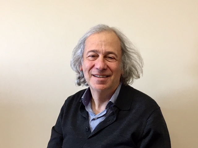
Pr Jacques Blum
Pr Jacques Blum — numerical analysis, control and data assimilation. From the École Normale Supérieure and a doctorate under Jacques-Louis Lions, through CNRS research and professorships at Grenoble, École Polytechnique and Nice, Jacques Blum built a career around the simulation, identification and optimal control of physical systems governed by partial differential equations.
His work spans tokamak plasma equilibrium, real-time reconstruction, ocean circulation and data assimilation. At DSTI he is a member of the Scientific Advisory Board and helped shape the school's approach to mathematical support across the student body. Distinctions include the CNRS Bronze Medal (1984), the Prix Blaise-Pascal (1990), the Seymour Cray prize (1998) and the Grand Prix de la Ville de Nice (2017).
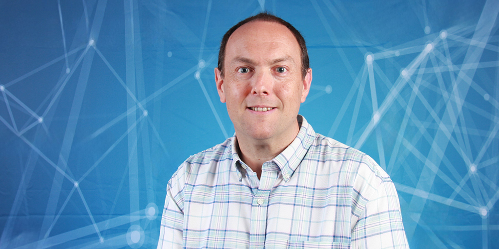
Pr Didier Auroux
Pr Didier Auroux — Director of the Maison de la Modélisation, de la Simulation et des Interactions. Didier Auroux trained at the École Normale Supérieure de Lyon and completed his doctorate under Jacques Blum's supervision — Étude de différentes méthodes d'assimilation de données pour l'environnement (2003) — followed by an habilitation on fast algorithms for image processing and data assimilation.
His research joins geophysics, observers, optimal control, inverse problems, numerical analysis and scientific computing. He now directs Université Côte d'Azur's Maison de la Modélisation, de la Simulation et des Interactions, a structure that supports research through modelling, simulation, high-performance computing and data science.
Both are attached to teaching across the full student population, including learners far from their own research level. Jacques proposed the creation of DSTI's Support Sessions, in the spirit of the recitation classes used at leading universities; Didier regularly leads support sessions for the mathematics-driven modules. Mathematical confidence is not created by lowering the intellectual ceiling. It is created by building a reliable route towards it — which is, in the end, what the course chain in §06 is.
06 The chain of teaching: from Applied Mathematics to Data Assimilation
What makes the DSTI version of this distinctive is not that two eminent mathematicians appear on a faculty list. It is that the same two people teach a connected sequence of courses, each a genuine prerequisite for the next, that carries a student from the gradient of a one-variable function to a working 4D-Var. Jacques Blum and Didier Auroux teach the three courses jointly, rotating the teaching days between them, so a cohort sees both professors throughout the chain rather than meeting one per subject. The destination is hard; the route is built deliberately.
Warm Up — Fundamentals of Mathematics. Every DSTI data MSc begins with a Warm Up that establishes the mathematical foundations, working with cohorts whose prior preparation varies widely. This is the levelling step before anything specialised.
Applied Mathematics for Data Science. Across the data MSc programmes, this course supplies the working mathematics that everything later assumes: differentiation in one and several variables, the gradient, Taylor expansion; linear algebra through vectors and matrices, linear systems, diagonalisation, eigenvalues and eigenvectors, and quadratic forms; and complex numbers. The syllabus is candid about its tools — "pen, paper and brain; R or Python to verify computations." These are not arbitrary topics: the gradient reappears as the object an optimiser follows, eigen-decomposition underlies covariance structure, and quadratic forms are the shape of every cost function in §04.
Continuous Optimisation. This is the hinge of the whole sequence. It develops cost functions and constraints (equality, inequality, and constraints given by a differential equation); Fréchet and Gâteaux differentiability; convexity; first- and second-order optimality conditions; the existence and uniqueness of a minimum — including the genuinely advanced material of minimisation in Hilbert spaces, weak convergence and lower-semicontinuity; Lagrange multipliers and duality; the Kuhn–Tucker (KKT) theorem and saddle points; and then the algorithms that do the work: gradient descent with fixed and optimal step, conjugate gradient, projected gradient and Uzawa's algorithm. Tellingly, the course already poses inverse problems as optimisation — among its worked examples are least squares (Av = b) and the identification of an unknown coefficient in −div(K∇u) = f by minimising J = Σ [u(xᵢ) − uᵢ]². The bridge to data assimilation is built into the optimisation syllabus itself.
Jacques proposed the creation of DSTI's Support Sessions, in the spirit of the recitation classes used at Ivy League and leading Californian universities. Didier regularly leads support sessions for mathematics-driven modules. The standard is high, and students are given additional structured teaching to help them reach it.
Inverse Problems & Data Assimilation. The research field enters the curriculum directly. The course covers well-posed versus ill-posed problems (Hadamard); variational methods (optimal control, the Lagrangian, adjoint methods); sequential methods (Kalman filtering); and nudging (observers). Its stated prerequisites are exact and unsentimental: "Maths, Continuous Optimisation & Python Labs," drawing also on the school's statistics and machine-learning foundations. The examples are parameter identification and model calibration — the same inverse-problem frame from §01, now at full strength.
Didier teaches Mathematics Harmonisation with Dr Christine Malot, helping students establish a shared mathematical foundation before progressing to later quantitative work. Explore the curriculum.
Jacques teaches the physics component, connecting computation to the physical systems, energy limits and environmental questions it affects. Explore the curriculum.
The laboratory work is where the article's own methods become something a student has built with their hands. The labs use the Lorenz system — the canonical low-dimensional chaotic model — in a twin-experiment design: generate a known "true" trajectory, create sparse noisy observations from it (observe two of the three variables, every hundred steps, with added noise), then start from a deliberately wrong background and try to recover the truth. On that single, honest test bed, students implement all three method families in turn:
- Nudging — forward then backward, i.e. BFN itself, coded directly;
- 4D-Var — the cost function, the adjoint model for its gradient, and the numerical gradient check before trusting it;
- Kalman — the linear filter, and then the Extended Kalman filter, which exposes exactly what breaks when a nonlinear model is forced through a linearised correction.
The twin experiment is itself a lesson in validation: because the truth is known by construction, every method can be scored against it — which is why it is the right place to learn, and also why it is easier than operational reality, where the truth is precisely what is missing. That gap between a diagnostic toy and the real system is named, not glossed over.
A note on the people behind the chain, because it is a real intellectual lineage and not a decoration. Jacques Blum completed his doctorate under Jacques-Louis Lions, whose optimal-control theory for systems governed by partial differential equations is the mathematical foundation on which 4D-Var rests. Didier Auroux, in turn, completed his doctorate under Jacques Blum — Étude de différentes méthodes d'assimilation de données pour l'environnement, defended in 2003. The optimal-control machinery taught in the data-assimilation course is, in a direct sense, the tradition the two of them inherited and extended — and the Back and Forth Nudging algorithm grew out of that same collaboration. The teaching chain, Lions → Blum → Auroux, recapitulates a research one.
The chain described here is the data-MSc spine, but it is not the whole of their teaching. At undergraduate level, Didier Auroux also teaches Mathematics Harmonisation in the BSc Computer Science & Engineering, with Dr Christine Malot, helping students build a shared mathematical footing before later quantitative work; and Jacques Blum teaches the physics of the BSc's Energy – Climate – Sustainable IT track, covered separately in Efficient IT begins before the code.
07 The scale problem, and why structure earns its place
It would be easy to mistake all of this for elegant theory. The course is emphatic that it is not, and the reason is scale. For atmosphere and oceans, a realistic grid has on the order of fifty vertical levels and several hundred points in each horizontal direction — well over ten million grid points — with several physical variables (velocity components, pressure, temperature, humidity or salinity, chemical concentrations) at each. The control vector for a 4D-Var can therefore reach 10⁷ to 10⁹ components; the number of observations is 10⁵–10⁶; the covariance matrices are nominally of size n × n, which is to say astronomically large; and an operational forecast centre must produce an analysis in three to six hours. Estimating the background-error covariance B at all is a research problem in its own right, and the forecast is sensitive to the choice.
This is the engineering reality behind the mathematics, and it is recognisably DSTI's territory — the place where memory, computational cost and a hard time budget decide which method is admissible. It is also why representing known structure is not a stylistic preference but an efficiency: a smaller, structured method can mean less data movement, less training, stronger physical consistency and a clearer account of failure than a larger generic learner. The discipline is to keep the boundary inspectable — to know which part of the system is being imposed from physics and which part is being learned from data.
Do not force the learner to rediscover what the domain already knows.
When reliable physical laws, constraints, taxonomies or relationships exist, represent them. Use data-driven learning for the residual uncertainty, unknown parameters, unresolved scales and patterns the explicit model cannot provide. Intelligence lies in the combination.
Conservation laws, differential equations, causal constraints and domain knowledge are information. Discarding them is not neutrality; it is a design decision.
Data are invaluable where parameters are uncertain, models are incomplete, sub-grid effects are unresolved or patterns cannot be specified analytically.
The difficult work is deciding how model error, observation error and learned components interact — and validating the resulting system.
Data assimilation
Combine a dynamical model with observations so the reconstructed state respects both the evidence and the laws governing evolution.
Semantic Web
Represent known entities and relationships explicitly rather than asking every downstream system to infer them repeatedly from unstructured data.
That principle echoes elsewhere in the curriculum — in Pr Fabien Gandon's teaching of Semantic Web technologies, the same instinct applied to knowledge rather than physics: represent what is already known explicitly, rather than systematically relearning the whole model from raw data. The shared discipline is to know what you know, learn what you do not, and make the boundary between them something you can inspect.
08 The research trail behind the classroom
The article is grounded in a sequence of publications that traces the work from the introduction of an algorithm and its convergence proof through numerical comparison, theoretical development and geophysical applications.
The founding note; introduces BFN and proves convergence for a linear ODE system.
Fuller development and numerical study in oceanographic assimilation.
The DBFN extension for diffusion in backward integration.
Tests on shallow-water and full ocean models, including behaviour under observation noise.
Foundations: inverse problems, optimal control, data assimilation
- Hadamard, J. (1902). Sur les problèmes aux dérivées partielles et leur signification physique. — The original definition of well-posedness.
- Lions, J.-L. (1971). Optimal Control of Systems Governed by Partial Differential Equations. Springer. — The optimal-control theory underlying variational data assimilation.
- Kalnay, E. (2003). Atmospheric Modeling, Data Assimilation and Predictability. Cambridge University Press. — Standard text; on the course reading list.
- Evensen, G. (2006). Data Assimilation: The Ensemble Kalman Filter. Springer. — Standard text; on the course reading list.
- Bennett, A. F. (2002). Inverse Modeling of the Ocean and Atmosphere. Cambridge University Press. — On the course reading list.
- Auroux, D. (2003). Étude de différentes méthodes d'assimilation de données pour l'environnement. Doctoral thesis, Université de Nice-Sophia Antipolis (supervised by Jacques Blum).
The professors
- Pr Jacques Blum — University page · Biography
- Pr Didier Auroux — University page · Publications · Maison de la Modélisation, de la Simulation et des Interactions
Material in §§01–07 describing the structure, scope and worked content of the courses (the inverse-problem framing and examples, the Hadamard well-posedness treatment and the differentiation instability, the 3D/4D-Var cost functions and the adjoint method, the discretise-versus-differentiate caution, the scale figures and operational constraints, the method taxonomy, and the Lorenz twin-experiment laboratories implementing nudging, 4D-Var and Kalman with a gradient check) is drawn from Professors Blum and Auroux's own DSTI course materials — the syllabi, lecture notes and student notebooks for Applied Mathematics for Data Science, Continuous Optimisation, and Inverse Problems & Data Assimilation — not public citations, except where a public source is linked inline.
Closing: the lesson students should keep
Artificial intelligence is not a single class of models. It is the disciplined construction of systems that infer, optimise and act under uncertainty. Sometimes data should learn the model. Sometimes data should correct a model that already encodes real physics. Knowing the difference — and being able to defend the choice with a cost function, an error covariance, a convergence argument and an honest account of what was assumed — is part of becoming an engineer who understands the scientific foundations rather than only the tools.
It is fitting that the course exists inside a chain that starts with the gradient of a single function and ends at a research frontier, taught by two mathematicians who learned the field from the person who largely founded its control-theoretic half. That is the version of expertise DSTI tries to teach: not the confidence to run a simulation, but the judgement to know what a reconstruction is worth.